Getting Started

Import the package specific classes and some helper packages for brevity.

matplotlib for plotting. jax.random to set the key (this is not required but highly encouraged). numpyro.distributions to initialise our priors (just for clarity) jax.numpy to initialise our kernel parametes (just for clarity)

from ife_surrogate.gp.models import WidebandGP
from ife_surrogate.gp.kernels import Kriging
from ife_surrogate.gp.trainers import SwarmTrainer

import matplotlib.pyplot as plt
import numpy as np
import jax.random as jr
import jax.numpy as jnp
from numpyro.distributions import Uniform, LogUniform

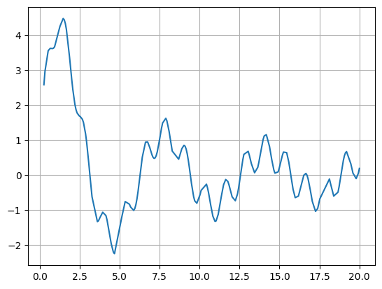
Next we generate some dummy data: (this is placeholder data until we find some data that better represents an actual usecase)

N = 300
X = np.linspace(0, 20, N)[:, None]
Y = np.sin(X) * 10 / (X + 1) + np.sin(X * 5) * 0.5

ii = np.random.permutation(N)
split = int(N * 0.5)
i_train, i_test = ii[:split], ii[split:]
i_train.sort()
i_test.sort()

x_train, y_train = X[i_train], Y[i_train]
x_test, y_test = X[i_test], Y[i_test]

plt.plot(x_train, y_train)
plt.grid()

We suggest a 3-Step-Workflow:

1. Kernel

The Kernel defines the spatial link between the data. To initialise the kernel requires defining the priors and the initial parameters. (This will likely be made easier in future versions.) Here we use a Kriging Kernel, which uses a “lengthscale” and a “power” hyperparameter.

d = x_train.shape[1]
priors = {"lengthscale" : Uniform(0, 1), "power" : LogUniform(0, 1)}
kernel = Kriging(lengthscale=jnp.ones(d), power=jnp.ones(d), priors=priors)

2. Model

The Model holds the objective function, which is already implemented. It only needs the training data and the kernel.

model = WidebandGP(x_train, y_train, kernel)

3. Trainer

After instantiating the model we need to train it. We provide two trainers, OptaxTrainer and SwarmTrainer. Both have a variety of settings, which are explored in Trainer Guide and in more detail in Trainers. (tldr; OptaxTrainer is really fast, but sometimes fails to yield a result, Swarmtrainer is slower but always converges)

trainer = SwarmTrainer()

best_run, history = trainer.train(model)

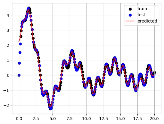
Afterwards you can use the model to predict on new data:

predictions, variances = model.predict(x_test)

plt.scatter(x_train, y_train, label="train", c="k")
plt.scatter(x_test, y_test, label="test", c="b")
plt.plot(x_test, predictions, label="predicted", c="r")
plt.grid()
plt.legend()
plt.show()